Quarto는 다음과 같은 콘텐츠를 작성할 수 있도록 다양한 페이지 레이아웃 옵션을 지원합니다.
- Fills the main content region
- Overflows the content region
- Spans the entire page
- Occupies the document margin
이 글에서는 페이지 여백에 콘텐츠를 배치하는 몇 가지 기능을 보여 줍니다. 전체 기능은 문서 레이아웃 가이드에서 확인하세요.
여백 그림
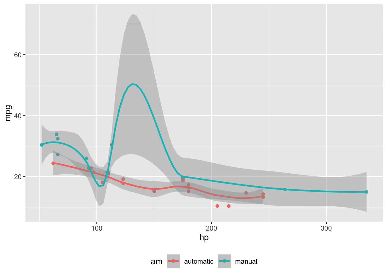
코드 셀로 생성한 그림은 column: margin 코드 셀 옵션을 사용해 여백에 배치할 수 있습니다. 코드가 둘 이상의 그림을 생성하면 각 그림이 여백에 배치됩니다.
```{r}
#| label: fig-mtcars
#| fig-cap: "MPG vs horsepower, colored by transmission."
#| column: margin

library(ggplot2)
mtcars2 <- mtcars
mtcars2$am <- factor(
  mtcars$am, labels = c('automatic', 'manual')
)
ggplot(mtcars2, aes(hp, mpg, color = am)) +
  geom_point() +
  geom_smooth(formula = y ~ x, method = "loess") +
  theme(legend.position = 'bottom')
```
여백 표
column: margin을 지정하면 문서 여백에 표를 배치할 수도 있습니다.
```{r}
#| column: margin

knitr::kable(
  mtcars[1:3, 1:3]
)
```| mpg | cyl | disp | |
|---|---|---|---|
| Mazda RX4 | 21.0 | 6 | 160 |
| Mazda RX4 Wag | 21.0 | 6 | 160 |
| Datsun 710 | 22.8 | 4 | 108 |
기타 콘텐츠
.column-margin 클래스를 가진 div로 여백 컬럼을 지정해 콘텐츠를 배치할 수도 있습니다. 예:
::: {.column-margin}
We know from *the first fundamental theorem of calculus* that for $x$ in $[a, b]$:

$$\frac{d}{dx}\left( \int_{a}^{x} f(u)\,du\right)=f(x).$$
:::
We know from the first fundamental theorem of calculus that for \(x\) in \([a, b]\):
\[\frac{d}{dx}\left( \int_{a}^{x} f(u)\,du\right)=f(x).\]
여백 참고
각주와 참고 문헌은 일반적으로 문서 끝에 나타나지만, 문서 front matter에 다음 옵션을 설정하면 여백에 표시되도록 할 수 있습니다.[^1]
---
reference-location: margin
citation-location: margin
---
이 옵션을 설정하면 각주와 인용(각각)이 페이지 하단이 아니라 문서 여백에 자동으로 배치됩니다. 예를 들어 Xie, Allaire, and Grolemund (2018) 을 인용하면, 해당 참고 문헌 항목이 여백에 나타납니다.
곁글
곁글(aside)은 본문 콘텐츠와 분리된 내용을 배치할 수 있게 해줍니다. 곁글은 각주처럼 보이지만 각주 표시(위첨자 번호)가 없습니다.
aside which places it in the margin without a footnote number.[This is a span that has the class aside which places it in the margin without a footnote number.]{.aside}여백 캡션
그림과 표의 경우 콘텐츠는 본문에 두고 캡션만 여백에 배치할 수 있습니다. 이를 제어하려면 코드 셀이나 문서 front matter에 cap-location: margin을 사용하세요. 예:
```{r}
#| label: fig-cap-margin
#| fig-cap: "MPG vs horsepower, colored by transmission."
#| cap-location: margin

library(ggplot2)
mtcars2 <- mtcars
mtcars2$am <- factor(
  mtcars$am, labels = c('automatic', 'manual')
)
ggplot(mtcars2, aes(hp, mpg, color = am)) +
  geom_point() +
  geom_smooth(formula = y ~ x, method = "loess") +
  theme(legend.position = 'bottom')
```